Press Release RBI Working Paper Series No. 03 Equity Markets and Monetary Policy Surprises Mayank Gupta, Amit Pawar, Satyam Kumar, Abhinandan Borad and Subrat Kumar Seet@ Abstract 1The paper examines the impact of monetary policy announcements on stock returns and volatility in equity prices in India. It decomposes changes in Overnight Indexed Swap (OIS) rates on policy announcement days into target and path factors. The target factor captures the surprise component in central bank policy rate action, while the path factor captures the impact of central bank communication on market expectations regarding the future path of monetary policy. The empirical analysis using daily data suggests that equity returns on policy announcement days are impacted only by the path factor (i.e., market’s expectations of future monetary policy trajectory), while both target and path factors (both of which capture the unanticipated component of monetary policy) impact the volatility in equity prices. An event study analysis undertaken by constructing short duration windows around the monetary policy announcements using intraday data also indicates that the path factor helps explain changes in equity returns. JEL Classification: C38, E52, E58 Keywords: Equity markets, monetary policy communication, principal component analysis Introduction How do equity markets react to monetary policy decisions? Is the reaction identical in case of a change in the policy rate versus no change in the policy rate? Does central bank’s communication have any bearing on the performance of the equity markets? This paper aims to answer these questions in the Indian context. Financial markets tend to react instantaneously with the release of new information and market prices reflect expectations about the future economic and monetary developments (Hildebrand, 2006). The financial market variables help to identify the immediate and more direct effect of changes in the monetary policy. Among various segments of the financial markets, asset prices, especially stock and bond prices, are regarded as being highly sensitive to any economic news. Financial market participants typically extract information from central bank’s monetary policy communication - announcements and decisions about the policy rate, policy stance, and assessment of current and future economic outlook. While establishing the link between monetary policy decisions and stock returns, one should account for the possibility that anticipated policy actions could have already been incorporated into market participants' decisions and only unanticipated changes would impact the markets. Unanticipated policy changes significantly impact both aggregate as well as the majority of the sectoral stock returns (Bredin et al., 2007). Monetary policy surprises are observed to have a statistically significant effect on both short and long-term risk-free rates (Ahmed et al., 2022)2. The Dividend Discount Model (DDM)3, which is widely used for equity valuation, stipulates that a rise in risk-free rate decreases equity prices and vice-versa (Gordon, 1962). Monetary policy announcements also provide information about the economic fundamentals called as the ‘information effect’ (Nakamura and Steinsson, 2018). Accordingly, in this paper, we focus on dissecting the unanticipated element (or ‘surprise’) of monetary policy and then understanding its linkage with the equity markets in the Indian context. A monetary policy surprise can be decomposed into: i) surprise in the current monetary policy rate action; and ii) surprise in the expected future path of monetary policy. The paper captures these two effects by constructing the target factor and the path factor, respectively, following two different methodologies: survey-based method (Andersson, 2010) and market-based method (Gurkaynak et al., 2004). The paper is organised as follows. Section II presents the background and related literature. Section III elaborates the methodology and results of the study. The intraday responses to monetary policy decisions are discussed in Section IV. Finally, Section V provides concluding observations. II. Literature Review Financial market participants keenly watch monetary policy announcements. While central bank communication and policy actions have the potential to impact various segments of financial markets, the scope of this paper is limited to their impact on equity markets. Bernanke and Kuttner (2005) find evidence of a strong and consistent stock market reaction to unexpected monetary policy actions in the US. Andersson (2010) using intraday data in the US and Euro area observes a sharp jump in intraday volatility at the time of the release of the monetary policy decisions. Rosa (2011) using high-frequency event study analysis in the US notes that the surprise component of both the central bank action and communication significantly impact equity indices. Lewis (2022) utilises US data spanning from 1996 to 2019 to identify distinct components of asset price changes resulting from monetary policy shocks. The analysis leverages the presence of heteroskedasticity in the intraday data to conduct announcement specific decompositions. The study finds that forward guidance and asset purchases have significant effects on yields, spreads, equities and uncertainty. Schmeling and Wagner (2019) document that the tone of the central bank communication matters for asset prices, and observe a strong link between the European Central Bank’s tone and equity prices. Lyocsa et al. (2019) observe high volatility in stock markets in G7 countries on the day of the announcement of monetary policy during 2006-2016. As regards India, Agrawal (2007), in his event study of the impact of monetary policy announcements on daily returns of NSE Nifty stocks, finds evidence on slow assimilation of information in stock prices, reflecting weak efficiency of stock markets in India. Sasidharan (2009) examines stock market behaviour on days preceding and succeeding the announcement of a change in the monetary policy stance using tests based on non-parametric statistics. It rejected any systematic difference in the return behaviour between expansionary and contractionary policy, as well as the days corresponding to the policy announcement event. Prabu et al. (2016) use 'event study' and 'identification through heteroscedasticity' methodology to study the impact of monetary policy announcements on stock indices during 2004–2014. The study does not find any statistically significant impact of monetary policy announcements on the stock indices. However, it finds evidence of a weakly significant impact of unexpected policy announcements, particularly on banking stocks. On the differential effects of monetary policy changes, Khuntia and Hiremath (2019) use Bloomberg surveys to decompose expected and unexpected components of policy changes and find a significant impact of unexpected monetary policy changes on stock market returns. By bifurcating monetary policy announcements into two factors, i.e., target factor – surprise change in the policy rate, and path factor – impact of changes in market’s expectations regarding the future path of the monetary policy, Gurkaynak et al. (2004) find that Federal Open Market Committee (FOMC) statements, rather than policy action, explain substantial variation in the movements of five and 10-year Treasury yields around FOMC meetings. In the Indian context, Lakdawala and Sengupta (2021) use changes in OIS rates around the monetary policy announcements to capture the unexpected (or surprise) component of the Monetary Policy Committee (MPC) decisions. Further, by using OIS rates of various maturities, they gauge the future path of policy rate from the Reserve Bank’s communication. The authors observe a significant impact of both target and path factors on India's stock market, with the target factor having a greater impact than the path factor. Ahmed et al. (2022), using daily data from October 2016 through April 2021, find that the association between monetary policy surprises and government as well as corporate bond yields across all maturities are positive and strong, while this is less evident for the exchange rate and stock prices in the Indian case. The paper contributes to the existing literature in two ways. First, we introduce the survey-based methodology for decomposing monetary policy decisions into target and path factors in the Indian context. Second, a tight window analysis of equity market reactions to monetary policy announcements using high-frequency intraday data is undertaken. III. Data and Methodology for Modelling of Monetary Policy Shocks Our analysis covers the period starting with the implicit adoption of a flexible inflation targeting regime in India, i.e., January 2014 and ends in July 20224. The data used to measure financial market reaction to policy announcements include daily data on OIS5 rates of all available maturities starting from one month up to one year and OHLC6 daily data on BSE Sensex. Further, as a proxy for the target factor, we use the difference between the mean estimate of the repo rate from the Bloomberg survey7 and the actual repo rate for each MPC announcement. All data, including survey data, are sourced from Bloomberg. OIS rates are frequently used to track changes in the future path of monetary policy rates. The OIS instruments are forward-looking and reflect the markets’ view of the likely Mumbai Interbank Outright Rate (MIBOR) in the future. We use MIBOR-linked OIS rate as an indicator of the markets’ prevailing view on the future path of monetary policy. For instance, the one-year OIS rate jumped in April 2022, as the Reserve Bank of India (RBI) changed its stance from ‘accommodative’ to ‘remain accommodative while focussing on the withdrawal of accommodation’ (Chart 1). It also introduced the standing deposit facility (SDF) at 25 basis points (bps) below the policy repo rate as the floor of the Liquidity Adjustment Facility (LAF) corridor, while reducing the width of the LAF corridor to 50 bps from 90 bps. The OIS rates reflect the totality of the changes in short-term funding conditions brought in by the RBI through the operation of various instruments, viz., repo rate, reverse repo rate, and cash reserve ratio (Lakdawala and Sengupta, 2021). In the study, we use 1 month, 3 months, 6 months, 9 months, 1 year and 5 year OIS rates to capture market expectations of funding conditions over various horizons8. The repo rate changes are most correlated with OIS 1 month (1M) rate changes (Chart 2). III.1 Descriptive Statistics Descriptive statistics for changes in OIS rates and Sensex on monetary policy announcement days are presented in Table 1. | Table 1: Descriptive Statistics | | Policy Days# | | | OIS1M | OIS3M | OIS6M | OIS9M | OIS1Y | OIS5Y | SENSEX | | Mean | 0.006 | -0.003 | 0.011 | 0.007 | 0.012 | 0.013 | -0.001 | | Standard Deviation | 0.12 | 0.11 | 0.14 | 0.14 | 0.14 | 0.12 | 0.01 | | Skewness | 0.37 | -0.33 | 2.48 | 2.21 | 2.09 | 0.66 | -0.13 | | Kurtosis | 2.98 | 1.51 | 12.31 | 9.78 | 8.65 | 0.86 | 0.97 | Note: For OIS rates, daily changes are presented, while for Sensex, return calculated using closing price is provided; Period: Jan 2014 – June 2022; Kurtosis figures are excess over normal.
#It includes 54 days, including unscheduled monetary policy announcements.
Source: Authors’ calculations. | Unscheduled policy announcements during the sample period have been highlighted in Chart 39 which presents the policy day changes in OIS rates and BSE Sensex. The sharpest movements in OIS rates in our sample were observed on the day of the unscheduled policy announcement on May 4, 2022. III.2 Methodology The OIS is a type of interest rate swap where the periodic fixed payments are tied to a given fixed rate, while the periodic floating payments are tied to a floating rate calculated from a daily compounded overnight MIBOR rate over the floating coupon period. The OIS rates have been found to accurately measure interest rate expectations for various countries (Lloyd, 2018). In the Indian context, the OIS rates of tenors 1, 9, and 12 months provide credible measures of market’s expectations of the future path of policy repo rate (Rituraj and Kumar, 2021). According to the theory of efficient markets, the expected policy announcement should have no impact on the OIS rates. Hence, in the absence of any other significant development, the changes observed in the OIS rates on policy announcement days could reflect the impact of the unexpected content of the policy announcement. Therefore, our identifying assumption is that fluctuations in the OIS rates on policy days are the result of the unanticipated content in policy announcement. A similar approach is taken by Nakamura and Steinsson (2018). The robustness of this assumption is tested by repeating the daily analysis on intraday data by creating tight windows of 30 and 60 minutes around policy announcements in the subsequent sections. Employing these insights, the study decomposes the policy-induced changes in the OIS rates into target factor (TF) and path factor (PF), where the former is intended to capture the impact of the unexpected repo rate changes on the OIS rates, while the latter captures the impact of changes in market expectations regarding the future path of the monetary policy. According to existing literature, this can be done either using financial market prices or through available surveys. Both methods have their advantages and disadvantages. Andersson (2010) points out that surveys are advantageous as they contain the actual mean expectations of the survey respondents about upcoming policy decisions and any deviations from that can be clearly interpreted as policy shocks. Measures derived from financial market expectations are beneficial as they are available at much higher frequency as compared to surveys. However, as Piazzesi and Swanson (2008) show that expectations derived from financial markets could be biased due to presence of risk premia and market noise. Taking cognisance of these practical issues, the study employs both the methodologies, viz., survey-based (Andersson, 2010) and market-based methods (Gurkaynak et al., 2005). III.2.1 Survey-based Method In the first method, the deviation of the mean survey10 responses from the actual repo rate is defined as the target factor. The path factor is then derived as the regression residual11 from a regression of OIS 1-Year rate on the estimated target factor as below: We have used the OIS 1-year rate as a proxy for monetary policy surprise because it is comparatively more liquid than other maturities. Further, the 1-year OIS also contains information on the future path of the monetary policy over a one-year horizon, which fits well with our objective of decomposing policy shocks into target and path factors. III.2.2 Market-based Method Principal components analysis (PCA) and linear algebra methods are used to decompose daily changes in the OIS rates of multiple maturities into the target and path factors. Consider a matrix W of daily changes in the OIS rates having maturities ranging from 1-month to 5 years on each of the announcement days. Given the discussion on the OIS rates as above and paying due consideration to the liquidity profile across maturities, this matrix W will contain information about the expectations of monetary policy for the horizon of up to 5 years. The size of W is t x n, where ‘t’ is the number of policy announcements, while ‘n’ is the number of instruments. W contains 54 policy announcements and 6 instruments, viz., 1 month, 3 months, 6 months, 9 months, 1 year and 5 year OIS rates in the present study. An arbitrary matrix W can be decomposed into a set of factors F of size t x m, such that m < n, with an error denoted by η. 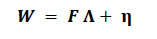 Following Gurkaynak et al. (2004), we used the Cragg and Donald (1997) rank test approach to find the number of dimensions of the monetary policy announcement for our sample, i.e., to test for the number of factors that explain the majority of changes in the OIS rates on policy days in a given sample period. In our sample period, monetary policy is characterised by two factors that explain the majority of the changes in the OIS rates (Table 2). | Table 2: Test for the Number of Factors Characterising Monetary Policy Announcements | | k0 factors | Chi-square degrees of freedom | Wald Statistics | p-value | Number of Observations | | 0 | 15 | 48.495 | 0.000 | 54 | | 1 | 9 | 20.645 | 0.014 | 54 | | 2 | 4 | 5.986 | 0.200 | 54 | Note: Cragg and Donald (1997) tests for the null hypothesis of k0 factors against the alternative of k > k0 factors for the underlying 54 x 6 matrix of OIS response to monetary policy announcement. For k0 = 2, we fail to reject the null hypothesis implying that two factors are sufficient to explain the response of OIS to monetary policy announcement.
Source: Authors’ calculations. | Accordingly, W is decomposed into two principal components, F1 and F2, which explain 94.4 per cent of the total variation in W12. By construction, these two factors are orthogonal, and hence, capture different aspects of the data. However, the two principal components lack any structural interpretation. Both F1 and F2 will be correlated with changes in the OIS 1-month rate. Hence, we cannot interpret the first factor as explaining the market's surprise to changes in the repo rate and the other factor to capture another dimension of the monetary policy. To address this, a rotation of the matrix F is performed to generate a new matrix Z, such that components of Z (i.e., Z1 and Z2) are orthogonal and explain the variation in W as well as F, but for which the second factor Z2 is uncorrelated with the changes in 1-month OIS rate. We define an orthogonal matrix U and can rewrite FɅ as FUU'Ʌ13. Now we have,  Such that Z & Ʌ* explain W as well as F and Ʌ. While there can be a large number of U matrices that satisfy the above condition, we need to identify U that allows a structural interpretation for Z such that the second column of Z (or the path factor) is a vector that is associated on average with no change in the 1-month OIS rate. We have four parameters, so we need four restrictions to identify U. The first two conditions come from simple normalisation imposed on the columns of U to have unit length. Next, we impose the following restriction to maintain the orthogonality condition, E(Z1Z2) = 0: Lastly, we impose the restriction that Z2 does not influence the current policy surprise i.e., changes in the 1-month OIS rate. Let γ1 and γ2 denote the (known) loadings of 1-month OIS rate on F1 and F2, respectively. The fourth condition is given as follows: It is easy to solve the unique matrix U satisfying these restrictions. Chart 4 shows the estimated target and path factors using the two methods. The left panels correspond to the target factor, while the right panels plot the path factor. The target and path factors derived from the two methods show moderate to high correlation of 0.66 and 0.82, respectively14. This deviation between the estimated factors may be due to the presence of risk premia and market noise in the market based methodology. III.3 Narrative Analysis In this section, we provide a brief narrative analysis of the estimated target and path factors and examine as to how the estimated values of the two factors align with the prevailing commentaries in the media. To achieve this, we collect policy dates with high absolute values of the estimated factors across both the methodologies as shown in Appendix Table A4. The highest values of the path factor through both the methodologies are observed on May 4, 2022. In an unscheduled monetary policy announcement on May 4, 2022, the Reserve Bank increased the policy repo rate under the LAF by 40 bps to 4.40 per cent. It was the first rate hike after maintaining a status quo in the policy repo rate in the previous 11 monetary policy announcements. The market interpreted the commentary by the Reserve Bank as an inflection point for further rate hikes in future meetings. It pointed towards a change in the future path of monetary policy, and so in our study, May 4, 2022, tops the list of absolute path factor values using both methods. The policy announcement on April 8, 2022 also shows high value of path factor as per both methods. Although the MPC kept the policy rate unchanged, it modified the stance “to remain accommodative while focussing on withdrawal of accommodation”, which was interpreted15 as the central bank’s pivot towards tightening in future policy announcements. Another unscheduled monetary policy announcement on March 27, 2020, features prominently in our list. This announcement was conducted in the backdrop of COVID-19, when the MPC decided to reduce the policy repo rate by 75 bps to 4.40 per cent from 5.15 per cent. A cut in the repo rate, the biggest absolute change in our study period, translated into a target surprise for the markets. Further, the MPC's commentary to “continue with the accommodative stance as long as it is necessary to revive growth and mitigate the impact of coronavirus (COVID-19) on the economy while ensuring that inflation remains within the target” was interpreted as the Reserve Bank’s resolve to support the economy through a prolonged period of accommodation. On December 5, 2019, the MPC left the repo rate unchanged - five successive rate cuts preceded this status quo in the policy repo rate. The Sensex declined marginally by 0.2 per cent. Similarly, the target factor showed a high value on October 5, 2018, another date when the MPC kept the repo rate unchanged. The repo rate was hiked in the previous two policy announcements, and the status quo surprised the market participants. During its second meeting on December 7, 2016, the MPC maintained status quo against an expected 25 bps cut in the repo rate. Finally, on September 29, 2015, the RBI reduced the repo rate by 50 bps from 7.25 per cent to 6.75 per cent, which came as a surprise for the market16. Equity markets gained on the policy announcement day. The above narrative broadly supports our empirical results. It may be noted that both our methods may not necessarily throw up the same dates17. As the two methods capture the monetary policy factors differently, some divergence may arise between their results18. Importantly, however, our results are able to capture revisions in the expectations of the future policy path quite well on dates of unscheduled monetary policy announcements. Any interpretation of the results can be potentially misleading if other significant macroeconomic data are released on the same day and at the same time around the MPC's monetary policy announcement. However, it may be noted that major macroeconomic data releases like inflation and GDP data are usually made after the 10th of every month, while most monetary policy announcements happen at the beginning of the month. Developmental and regulatory measures, and liquidity management and other financial market-related announcements, by the Reserve Bank are made simultaneously along with monetary policy announcements and these can also impact markets. Further, global developments might also impact markets in addition to policy actions. III.4 Results We estimate the impact of the two extracted factors on the returns and volatility of Sensex using the following equations: where Rt is the daily return on Sensex, TFt is the target factor at time t and PFt is the path factor at time t19. We also check for the impact of these two factors on the daily volatility in the Sensex. The volatility measure is derived as the logarithmic difference between the daily high and low prices (Alizadeh et al., 2002). Further, to capture the impact of monetary policy surprises on the Sensex returns and volatility conditional on the MPC changing the repo rate, we run two more regressions using the dummy variable approach, as suggested by Andersson (2010), where, D is a dummy variable (D is 1 when MPC alters the policy rate and zero when rates are kept constant) and X is a T x 2 matrix containing the target and path factors, such that T is the number of policy announcements in the sample. 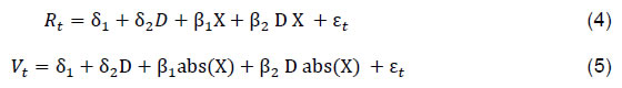
| Table 3: Regression Results | | Variables | Survey-Based | Market-Based | | Rt | Vt | Rt | Vt | | Intercept | -0.001 | 0.009*** | -0.001 | 0.010*** | | | (0.001) | (0.001) | (0.001) | (0.001) | | PF | -0.020** | | -0.004*** | | | | (0.009) | | (0.001) | | | TF | -0.003 | | 0.000 | | | Abs(PF) | (0.007) | 0.018*** | (0.001) | 0.003* | | | | (0.006) | | (0.002) | | Abs(TF) | | 0.040*** | | 0.002** | | | | (0.010) | | (0.001) | | Observations | 54 | 54 | 54 | 54 | | Adjusted R2 | 0.015 | 0.496 | 0.035 | 0.099 | | F Statistic | 2.797* | 19.458*** | 3.770** | 4.025** | Note: * : p<0.1; ** : p<0.05; *** : p<0.01; Newey-West standard errors are in parentheses.
Source: Authors’ calculations. | According to the regression analysis, first, repo rate surprises, as captured by the target factor, have almost no effect on equity returns. The market’s expectations of the future path of monetary policy, as captured by the path factor, however, remain significant. This corroborates the conventional thinking that markets are forward-looking, and the expected path of monetary policy could have implications for the cost of capital for corporates, affecting future earnings, and hence, equity returns (Table 3). Second, equity markets' volatility is affected by both the target and path factors, as markets digest the policy announcements throughout the day and traders adjust their portfolios (Table 3). Third, to check for the asymmetric impact of a repo rate change versus no change, the alternative specifications as per equations (4) and (5) were used. The results are in accordance with the baseline specifications and fit the data better as observed in significantly higher adjusted R2. The results suggest that stock prices react differently when policy rates are altered compared with when policy rates are left unchanged. For returns, an increased negative asset price sensitivity with respect to the path factor is observed when the repo rate is altered. For volatility, the sensitivity to the path factor continues to be significant, however, target factor is found to be insignificant (Table 4). | Table 4: Regression Results Conditional on Altered Repo Rate | | Variables | Survey-Based | Market-Based | | Rt | Vt | Rt | Vt | | Intercept | D = 1 | -0.006* | -0.001 | -0.006** | 0.001 | | | (0.003) | (0.003) | (0.003) | (0.003) | | Intercept | 0.002 | 0.010*** | 0.002 | 0.010*** | | | (0.001) | (0.001) | (0.001) | (0.001) | | PF | D = 1 | -0.032* | | -0.005** | | | TF | D = 1 | (0.017) | | (0.002) | | | Abs(PF) | D = 1 | | 0.002 | | 0.008** | | | | (0.014) | | (0.003) | | Abs(TF) | D = 1 | | 0.034 | | 0.002 | | PF | -0.000 | (0.021) | -0.000 | (0.001) | | TF | (0.011) | | (0.002) | | | Abs(PF) | | 0.015*** | | -0.003 | | | | (0.004) | | (0.003) | | Abs(TF) | | 0.011 | | 0.001 | | | | (0.015) | | (0.001) | | Observations | 54 | 54 | 54 | 54 | | Adjusted R2 | 0.109 | 0.518 | 0.138 | 0.261 | | F Statistic | 5.549*** | 12.840*** | 15.018*** | 12.836*** | Note: * : p<0.1; ** : p<0.05; *** : p<0.01; Newey-West standard errors are in parentheses.
. | D = 1 signifies the coefficient on dummy interaction terms; Regression specifications are as per (4) & (5).
Source: Authors’ calculations. | IV. Intraday Response to Monetary Policy The analysis using intraday data provides an advantage of constructing tight windows around the policy announcements. Measuring changes in a narrow window of time (say an hour or less) around policy announcements makes it less likely that any other significant macroeconomic event may have taken place during that time which may have influenced the asset prices (Gurkaynak et al., 2004). Thus, the high frequency approach can also act as another robustness check for our earlier findings using daily data. Due to data availability issues, the sample period for this exercise is June 6, 2018 - June 22, 2022, which includes 26 MPC meetings (23 scheduled and 3 unscheduled). One data point of March 27, 2020 has been eliminated from our sample, as it was a major outlier, given extreme COVID-19 related uncertainty. As in the daily analysis, changes in the 1-year OIS rate are used as a proxy for the monetary policy surprise. The 5-minute interval intraday data for 1-year OIS was obtained from Clearing Corporation of India Limited (CCIL), while corresponding interval data on Sensex was sourced from Bombay Stock Exchange (BSE). Tight windows were created around the policy announcement. Gurkaynak et al. (2004) use two windows of sizes 30 minutes (60 minutes), which begin 10 minutes (15 minutes) before the policy announcement, and end 20 minutes (45 minutes) after the announcement. Similarly, Swanson (2021) uses a 30 minute window around the announcement. One complication that can arise in using the intraday data could be the sparse trading in OIS contracts. This implies that there may be policy days when trades did not occur within the selected windows. To address this, we follow Gurkaynak et al. (2004) to take the first trade after the end of the window, and calculate the change from the prevailing rate at the start of the window. IV.1 Statistical Analysis The correlation coefficient between the Sensex returns and the change in 1-year OIS rates varies across windows; it is negative and statistically significant only in the tight window (Table 5). In the wide window, the correlation is statistically not significant. | Table 5: Correlation between the BSE Sensex Returns and Changes in OIS 1-Year | | Windows | Tight Window (30 minutes) | Wide Window (60 minutes) | | Correlation Coefficient between returns and change in 1 year OIS | -0.374* | -0.189 | | (-1.934) | (-0.921) | Note: Significance level: ‘***’ 0.01 (1%), ‘**’ 0.05 (5%), ‘*’ 0.1 (10%). t-statistics are reported in parentheses.
Source: Authors’ calculations. | IV.2 Impact of Monetary Policy Changes on Sensex Returns We follow the survey-based method for intraday analysis as described in Section III.2.1 but instead of daily changes, we use changes in 1-year OIS rates during 30 minutes (5 minutes before and 25 minutes after the policy announcement) and 60 minutes (5 minutes before and 55 minutes after the policy announcement). First, we regress the changes in the 1-year OIS rates in a tight window (30 or 60 minutes) on the surprise or the target factor, i.e., the deviation of the mean survey responses from the announced repo rate. The residuals are referred to as the path factor. Secondly, we estimate the following equation: where the δ, t subscript signifies the changes in a window δ on policy day t. Results are presented in Table 6. The market-based method cannot be applied here due to the sparse trading in OIS of maturity of less than 1 year during the 30 and 60 minutes intervals around the announcement, as noted earlier. Our results indicate that the path factor inversely affects Sensex returns in both tight as well as wide windows. The target factor does not show any significant impact on Sensex returns. | Table 6: Response of BSE Sensex Returns to Announcements | | Variables | Tight Window
(30 minutes) | Wide Window
(60 minutes) | | Constant | 0.00 | -0.001 | | (0.001) | (0.001) | | PF | -0.024** | -0.044** | | (0.007) | (0.013) | | TF | 0.001 | 0.010 | | (0.003) | (0.009) | | Observations | 25 | 25 | | Adjusted R2 | 0.275 | 0.298 | | F statistics | 5.559*** | 6.087*** | Note: Significance level: ‘***’ 0.01 (1%), ‘**’ 0.05 (5%), ‘*’ 0.1 (10%). Standard errors are reported in parentheses. Newey-West standard errors are in parentheses.
Source: Authors’ calculations. | V. Conclusions The study examines the response of equity markets to monetary policy surprises. Using the OIS rates as a measure of market’s expectations about the future path of monetary policy, we construct policy surprise as changes in the OIS rates around announcements. Statistical tests show that two factors are sufficient to explain the changes in the OIS rates. Using this cue, we decompose changes in the OIS rates on policy days into target and path factors, where the former is intended to capture the impact of the unanticipated repo rate change on equity markets, while the latter captures the changes in the market’s expectation of the future monetary policy trajectory. The paper’s analysis suggests that equity markets are affected more by the changes in the market’s expectations of future monetary policy (path factor) than the policy rate surprise (target factor) which is in agreement with the conventional thinking that equity markets are forward-looking. We also find that volatility in equity markets is affected by both target and path factors, as markets digest the policy announcements and traders adjust their portfolios throughout the day. Using an alternative specification to examine the potential asymmetric impact, we find an increased negative sensitivity of equity returns with respect to the path factor when repo rate is altered vis-à-vis when the rate is left unaltered. For volatility, the sensitivity to the path factor continues to be significant. While the intraday analysis with narrow windows of 30 and 60 minutes is aimed at controlling for other potential drivers of equity prices, it may be noted that the monetary policy announcements are accompanied by regulatory and developmental measures which can also impact markets. The sparse trading on occasions in the OIS markets as well as other domestic and global developments during the narrow window can also impact the analysis.
References Agrawal, G. (2007). Monetary policy announcements and stock price behavior: empirical evidence from CNX Nifty. Decision (0304-0941), 34(2). Ahmed, F., Binici, M., & Turunen, J. (2022). Monetary policy communication and financial markets in India. IMF Working Papers, 2022(209). Alizadeh, S., Brandt, M. W., & Diebold, F. X. (2002). Range‐based estimation of stochastic volatility models. The Journal of Finance, 57(3), 1047-1091. Anderson, M. (2010). Using intraday data to gauge financial market response to federal reserve and ECB monetary policy decision. International Journal of Central Banking, 6(2), 107-116. Bernanke, B. S., & Kuttner, K. N. (2005). What explains the stock market's reaction to federal reserve policy?. The Journal of Finance, 60(3), 1221-1257. Bredin, D., Hyde, S., Nitzsche, D., & O'reilly, G. (2007). UK stock returns and the impact of domestic monetary policy shocks. Journal of Business Finance & Accounting, 34(5‐6), 872-888. Cragg, J. G., & Donald, S. G. (1997). Inferring the rank of a matrix. Journal of Econometrics, 76(1-2), 223-250. Gordon, M. J. (1962). The Savings, investment, and valuation of a corporation. Review of Economics and Statistics, pp. 37-51. Gurkaynak, R. S., Sack, B., & Swanson, E. T. (2004). Do actions speak louder than words? The response of asset prices to monetary policy actions and statements. Finance and Economics Discussion Series, 2004(66), 1–43. Hildebrand, P. M. (2006). Monetary policy and financial markets. Financial Markets and Portfolio Management, 20(1), 7-18. Khuntia, S., & Hiremath, G. S. (2019). Monetary policy announcements and stock returns: some further evidence from India. Journal of Quantitative Economics, 17, 801-827. Lakdawala, A., & Sengupta, R. (2021). Measuring monetary policy shocks in India. Indira Gandhi Institute of Development Research Working Paper,(2021-021). Lewis, Daniel J. (2022). Announcement-specific decompositions of unconventional monetary policy shocks and their macroeconomic effects. Federal Reserve Bank of New York Staff Reports, (891). Lloyd, S. (2018), Overnight index swap market-based measures of monetary policy expectations. Bank of England Working Paper,(709). Lyócsa, Š., Molnár, P., & Plíhal, T. (2019). Central bank announcements and realized volatility of stock markets in G7 countries. Journal of International Financial Markets, Institutions and Money, 58, 117-135. Nakamura, E., & Steinsson, J. (2018). High-frequency identification of monetary non-neutrality: the information effect. The Quarterly Journal of Economics, 133(3), 1283-1330. Piazzesi, M., & Swanson, E. T. (2008). Futures prices as risk-adjusted forecasts of monetary policy. Journal of Monetary Economics, 55(4), 677-691. Prabu, E., Bhattacharyya, I., & Ray, P. (2016). Is the stock market impervious to monetary policy announcements: evidence from emerging India. International Review of Economics & Finance, 46, 166-179. Rituraj, & Kumar, A. V. (2021). Assessing the market’s expectations of monetary policy in India from overnight indexed swap rates. RBI Bulletin February, pp. 73-84. Rosa, C. (2011). Words that shake traders: the stock market's reaction to central bank communication in real time. Journal of Empirical Finance, 18(5), 915-934. Sasidharan, Anand. (2009). Stock market's reaction to monetary policy announcements in India. Munich Personal RePEc Archive Paper 24190. Schmeling, M., & Wagner, C. (2019). Does central bank tone move asset prices?. Available at SSRN 2629978. Swanson, E. T. (2021). Measuring the effects of federal reserve forward guidance and asset purchases on financial markets. Journal of Monetary Economics, 118, 32-53.
Appendix | Table A1: RBI Monetary Policy Decisions | | Total number of events | 54 | | Number of events in which the repo rate was changed | 19 | | Number of events in which the repo rate was left unchanged | 35 | | Number of increases, 25 bps | 3 | | Number of decreases, 25 bps | 10 | | Number of decreases, 35 bps | 1 | | Number of increases, 50 bps | 1 | | Number of decreases, 50 bps | 1 | | Number of increases, 40 bps | 1 | | Number of decreases, 40 bps | 1 | | Number of decreases, 75 bps | 1 | | Source: Authors’ calculations. |
| Table A2: Bloomberg Surveys of All Announcements | | Date | Change in Repo Rate (in bps) | New Repo Rate (%) | Median (%) | Average (%) | No. of Economists Surveyed | S.D (%) | | Jan 28, 2014 | 25 | 8 | 7.75 | 7.77 | 45 | 0.06 | | Apr 01, 2014 | 0 | 8 | 8 | 8.02 | 39 | 0.07 | | Jun 03, 2014 | 0 | 8 | 8 | 8 | 38 | 0 | | Aug 05, 2014 | 0 | 8 | 8 | 7.99 | 41 | 0.05 | | Sep 30, 2014 | 0 | 8 | 8 | 8 | 51 | 0 | | Dec 02, 2014 | 0 | 8 | 8 | 7.98 | 48 | 0.07 | | Jan 15, 2015* | -25 | 7.75 | | 8 | 0 | 0 | | Feb 03, 2015 | 0 | 7.75 | 7.75 | 7.69 | 41 | 0.11 | | Mar 04, 2015* | -25 | 7.5 | | 7.75 | 0 | 0 | | Apr 07, 2015 | 0 | 7.5 | 7.5 | 7.45 | 42 | 0.1 | | Jun 02, 2015 | -25 | 7.25 | 7.25 | 7.29 | 41 | 0.1 | | Aug 04, 2015 | 0 | 7.25 | 7.25 | 7.23 | 42 | 0.06 | | Sep 29, 2015 | -50 | 6.75 | 7 | 7.04 | 52 | 0.1 | | Dec 01, 2015 | 0 | 6.75 | 6.75 | 6.75 | 47 | 0 | | Feb 02, 2016 | 0 | 6.75 | 6.75 | 6.74 | 44 | 0.05 | | Apr 05, 2016 | -25 | 6.5 | 6.5 | 6.49 | 42 | 0.09 | | Jun 07, 2016 | 0 | 6.5 | 6.5 | 6.5 | 44 | 0 | | Aug 09, 2016 | 0 | 6.5 | 6.5 | 6.48 | 29 | 0.06 | | Oct 04, 2016 | -25 | 6.25 | 6.5 | 6.38 | 39 | 0.14 | | Dec 07, 2016 | 0 | 6.25 | 6 | 6.02 | 44 | 0.13 | | Feb 08, 2017 | 0 | 6.25 | 6 | 6.03 | 39 | 0.08 | | Apr 06, 2017 | 0 | 6.25 | 6.25 | 6.25 | 52 | 0 | | Jun 07, 2017 | 0 | 6.25 | 6.25 | 6.24 | 50 | 0.05 | | Aug 02, 2017 | -25 | 6 | 6 | 6.07 | 57 | 0.11 | | Oct 04, 2017 | 0 | 6 | 6 | 5.99 | 32 | 0.04 | | Dec 06, 2017 | 0 | 6 | 6 | 5.97 | 48 | 0.08 | | Feb 07, 2018 | 0 | 6 | 6 | 6.01 | 33 | 0.04 | | Apr 05, 2018 | 0 | 6 | 6 | 6 | 42 | 0 | | Jun 06, 2018 | 25 | 6.25 | 6 | 6.08 | 44 | 0.12 | | Aug 01, 2018 | 25 | 6.5 | 6.5 | 6.44 | 53 | 0.11 | | Oct 05, 2018 | 0 | 6.5 | 6.75 | 6.7 | 49 | 0.1 | | Dec 05, 2018 | 0 | 6.5 | 6.5 | 6.52 | 52 | 0.07 | | Feb 07, 2019 | -25 | 6.25 | 6.5 | 6.44 | 43 | 0.11 | | Apr 04, 2019 | -25 | 6 | 6 | 6.01 | 47 | 0.05 | | Jun 06, 2019 | -25 | 5.75 | 5.75 | 5.76 | 43 | 0.12 | | Aug 07, 2019 | -35 | 5.4 | 5.5 | 5.5 | 40 | 0.07 | | Oct 04, 2019 | -25 | 5.15 | 5.15 | 5.11 | 39 | 0.07 | | Dec 05, 2019 | 0 | 5.15 | 4.9 | 4.89 | 43 | 0.05 | | Feb 06, 2020 | 0 | 5.15 | 5.15 | 5.15 | 37 | 0 | | Mar 27, 2020* | -75 | 4.4 | NA | NA | 0 | NA | | May 22, 2020* | -40 | 4 | NA | NA | 0 | NA | | Aug 06, 2020 | 0 | 4 | 3.75 | 3.86 | 44 | 0.14 | | Oct 09, 2020 | 0 | 4 | 4 | 4 | 32 | 0 | | Dec 04, 2020 | 0 | 4 | 4 | 4 | 32 | 0 | | Feb 05, 2021 | 0 | 4 | 4 | 3.94 | 35 | 0.13 | | Apr 07, 2021 | 0 | 4 | 4 | 4 | 30 | 0 | | Jun 04, 2021 | 0 | 4 | 4 | 4 | 44 | 0 | | Aug 06, 2021 | 0 | 4 | 4 | 4 | 29 | 0 | | Oct 08, 2021 | 0 | 4 | 4 | 4 | 34 | 0 | | Dec 08, 2021 | 0 | 4 | 4 | 4 | 35 | 0 | | Feb 10, 2022 | 0 | 4 | 4 | 4.01 | 39 | 0.04 | | Apr 08, 2022 | 0 | 4 | 4 | 4 | 36 | 0 | | May 04, 2022* | 40 | 4.4 | NA | NA | 0 | NA | | Jun 08, 2022 | 50 | 4.9 | 4.8 | 4.83 | 41 | 0.1 | Note: * = Unscheduled Monetary Policy announcements; NA = Not Applicable
Source: Compiled by Authors. |
| Table A3: Principal Component Analysis of Changes in OIS Rates | | PC | Explained Variance (%) | | PC 1 | 87.5 | | PC 2 | 6.9 | | PC 3 | 4.1 | | PC 4 | 1.0 | | PC 5 | 0.4 | | PC 6 | 0.1 | | Source: Authors’ calculations. |
| Table A4: Dates of Top Five Target and Path Factors | | Target Factor | Path Factor | | Survey method | Market method | Survey method | Market method | | March 27, 2020 | December 07, 2016 | May 4, 2022 | May 4, 2022 | | May 4, 2022 | September 29, 2015 | April 8, 2022 | April 8, 2022 | | May 22, 2020 | October 5, 2018 | February 10, 2021 | December 7, 2016 | | September 29, 2015 | December 5, 2019 | March 27, 2020 | June 3, 2014 | | December 05, 2019 | March 4, 2015 | June 3, 2014 | April 4, 2019 | | Source: Authors’ calculations. |
| Table A5: Regression Results after Controlling for Overnight Global Developments | | Variables | Survey-Based | Market-Based | | Rt | Rt | | Intercept | -0.001 | -0.001 | | | (0.001) | (0.001) | | PF | -0.022** | -0.004*** | | | (0.009) | (0.001) | | TF | -0.002 | 0.000 | | | (0.009) | (0.001) | | Lagged S&P 500 | 0.081 | 0.053 | | | (0.102) | (0.101) | | Observations | 54 | 54 | | Adjusted R2 | 0.006 | 0.076 | | F Statistic | 2.282* | 2.507* | Note: * : p<0.1; ** : p<0.05; *** : p<0.01; Newey-West standard errors are in parentheses.
Source: Authors’ calculations. |
|